10 Google Sheets Formulas Every SEO Should Know

I’m sure most of you are somewhat familiar with Sheets (if not, it’s basically just like Excel, but cloud-based and completely free) and know just how powerful it can be when it comes to collaboration.

But, its capabilities reach far beyond collaboration.

Google Sheets can be used to scrape data from websites, create semi-automated SEO workflows, manipulate big data sets (e.g. a Site Explorer export), automate follow-ups for outreach campaigns, and much more.

In this post, I’ll introduce you to 10 Google Sheets formulas and show how you can use them for everyday SEO tasks.

Let’s start with the basics…

In this short section, I’m going to share three basic must-know formulas.

No matter what kind of SEO work I’m doing in Google Sheets, I find myself using these three formulas (almost) every time:

• IF;
• IFERROR;
• ARRAYFORMULA

Let’s start with an IF statement.

This is super simple; it’s used to check if a condition is true or false.

Syntax: =IF(condition, value_if_true, value_if_false)

Here’s an example spreadsheet containing a list of keywords with their respective estimated search volumes (note: these were gathered using Keyword Explorer):

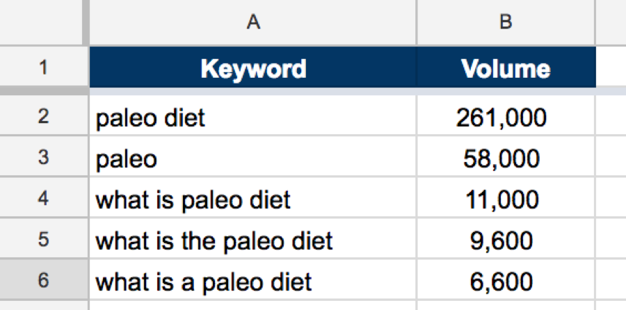
Let’s assume, hypothetically, that we have a strong site capable of ranking #1 for any of these keywords. However, we only want to go after keywords that are likely to bring in 500+ visitors per month (assuming we have a #1 ranking).

According to this study, #1 rankings in the US (desktop searches only) have a 29% CTR, roughly.

So, let’s write an IF statement that will return “GOOD” for keywords that are likely to bring 500+ visitors (i.e. those where 29% of the search volume is bigger than or equal to 500) and “BAD” for the rest.

Here’s the formula:

=IF(B2*0.29>=500,"GOOD","BAD")

Here’s what this does (in plain English):

1. It checks to see if B2*0.29 (i.e. 29% of the search volume) is bigger than or equal to 500;
2. If the condition is true, it returns “GOOD”. If it’s false, it returns “BAD”.

This works very well for our current data set, but look what happens when we throw some non-numerical values into the mix:

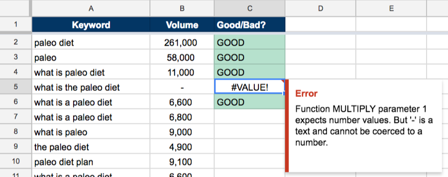
That’s an error.

This happens because it’s impossible to multiply a non-numerical value by 0.29 (obviously).

This is where IFERROR comes in handy.

IFERROR allows you to set a default value should the formula result in an error.

Syntax: =IFERROR(original_formula, value_if_error)

Let’s incorporate this into the example above (we’ll leave the cell blank if there’s an error) and see what happens:

Perfect — that’s the formula complete!

OK, so if you only ever work with a tiny amount of data, feel free to skip straight to the next section.

But, given the fact that this guide is for SEO’s, I’m going to assume that you’re working with reasonably large amounts of data on a regular basis.

If this is the case, I’d hazard a guess that you spend far too much time dragging formulas down across hundreds, possibly even thousands, of cells.

Enter: ARRAYFORMULA.

Syntax: =ARRAYFORMULA(array_formula)

Basically, an ARRAYFORMULA converts your original formula into an array, thus allowing you to iterate the same formula across multiple rows by writing only a single formula.

So, let’s delete all formulas in cells B2 onwards, and wrap the entire formula currently in cell B1 in an ARRAYFORMULA, like so:

=ARRAYFORMULA(IFERROR(IF(B2:B29*0.29>=500,"GOOD","BAD"),""))

Magic.

That’s the basics covered; let’s take a look at some more useful formulas.

1. Use REGEXTRACT to extract data from strings

REGEXTRACT uses regular expressions to extract substrings from a string or cell.

Syntax: =REGEXEXTRACT(text, regular_expression)

Here are just a handful of potential use cases for this:

• Extract domain names from a list of URLs (keep reading to see an example!);
• Extract the URL (i.e. without the root domain);
• Check if URL uses HTTP or HTTPS;
• Extract email addresses from a big chunk of text;
• Identify URLs with/without certain words in them from a list of URLs (e.g. URLs containing the “/category/guest-post” slug).

Let’s assume we want to extract the root domains from a list of “write for us” page URLs (i.e. guest post opportunities).

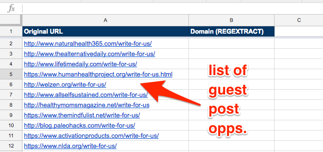
In column B, we can write a REGEXTRACT formula to do this.

Here is the regex syntax we need: ^(?:https?:\/\/)?(?:[^@\n]+@)?(?:www\.)?([^:\/\n]+)

Here’s our final formula:

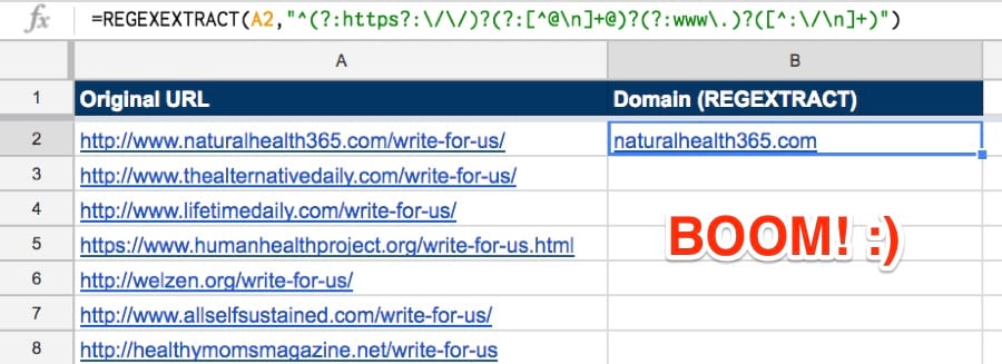
=REGEXEXTRACT(A2,"^(?:https?:\/\/)?(?:[^@\n]+@)?(?:www\.)?([^:\/\n]+)")

Paste this into cell B2 and, hey presto, we’ve extracted the domain.

Let’s wrap this in an ARRAYFORMULA and IFERROR to complete the entire column.

=IFERROR(ARRAYFORMULA(REGEXEXTRACT(A2:A,"^(?:https?:\/\/)?(?:[^@\n]+@)?(?:www\.)?([^:\/\n]+)")),"")

2. SPLIT strings into multiple data points

SPLIT divides (i.e. splits) strings into fragments using a delimiter.

Syntax: =SPLIT(text, delimiter)

Here are just a handful of potential use cases for this:

• Split a prospect’s full name into “first name” and “last name” columns;
• Split a URL into 3 columns for HTTP protocol, root domain, and URL slug;
• Split a list of comma-separated values into multiple columns;
• Split a root domain into 2 columns for domain name and domain extension (e.g. .com, .org, etc.)

I have a nice list of Ahrefs’ team members (full names) in a spreadsheet.

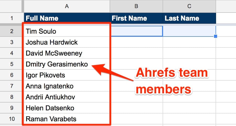
Here’s a simple SPLIT formula we could use in cell B2 to divide these into first name and last name:

=SPLIT(A2," ")

Again, let’s wrap this in an IFERROR and ARRAYFORMULA to split the entire list with a single formula.

=IFERROR(ARRAYFORMULA(SPLIT(A2:A," ")),"")

Here’s another example formula that will split root domains into site name and domain extension:

=SPLIT(A2,".")

3. Merge multiple data sets using VLOOKUP

VLOOKUP allows you to search a range using a search key—you can then return matching values from a specific cell in said range.

Syntax: =VLOOKUP(search_key, range, index_key)

Here are just a handful of potential use cases for this:

• Merging data from multiple sources (e.g. merging a list of domains with corresponding Ahrefs DR ratings from a separate sheet);
• Checking if a value exists in another data set (e.g. checking for duplicates across two or more lists of outreach prospects);
• Pulling in email addresses (from a master database of contacts) alongside a list of prospects.

Let’s assume we have a list of outreach prospects (i.e. a bunch of people linking to a competitor’s website, pulled from Site Explorer). We also have a master database of contact information (i.e. email addresses) in another spreadsheet.

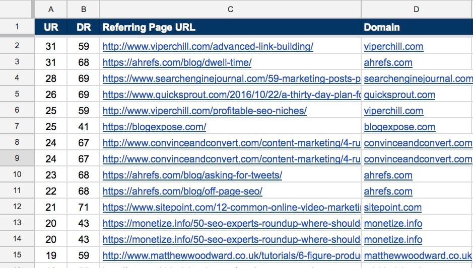
Site Explorer export (note: I removed many of the columns here, as much of the data isn’t needed for this example).

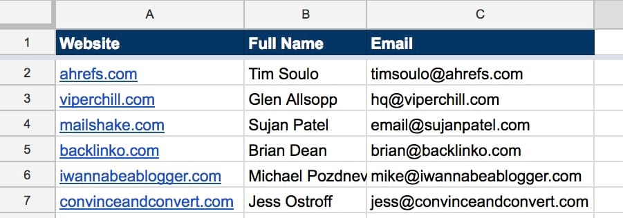
Master contact database — this is the database we’ll be querying using a VLOOKUP function.

We don’t want to waste time looking for contact information that we already have, so let’s use VLOOKUP to query the master database and see if we already have contact info for any of these prospects.

Here’s the formula we’re going to use:

=VLOOKUP(D2:D,'Master contact database'!A:C,2)

OK, let’s do the same for the email column; we’ll also wrap both formulas in an IFERROR and ARRAYFORMULA.

=IFERROR(ARRAYFORMULA(VLOOKUP(D2:D,'Master contact database'!A:C,3)),"")

4. Scrape data from any website using IMPORTXML

IMPORTXML lets you import data (using an XPath query) from a number of structured data types including XML, HTML, and RSS (amongst others).

In other words, you can scrape the web without ever leaving Google Sheets!

Syntax: =IMPORTXML(url, xpath_query)

Here are just a handful of potential use cases for this:

• Scraping metadata from a list of URLs (e.g. title, description, h‑tags, etc);
• Scraping email addresses from web pages;
• Scraping social profiles (e.g. Facebook) from web pages;
• Scraping lastBuildDate from RSS feeds (this is a really sneaky way to see how recently the site was updated without even having to load the website!)

Let’s assume that we wanted to grab the meta title for our post about keyword research.

We can see in the HTML that the meta title reads: “How To Do Keyword Research in 2017 — Ahrefs’ Guide”.

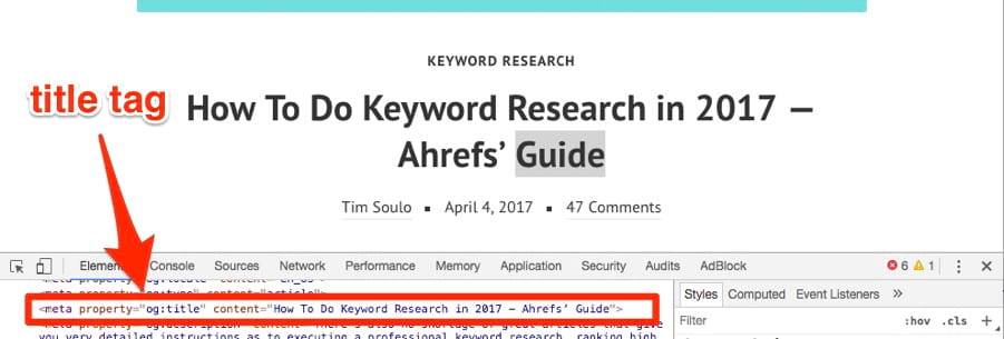
The XPath query we use to grab the meta title is quite simply: “//title”

Here’s the formula:

=IMPORTXML("https://ahrefs.com/blog/keyword-research/","//title")

It’s also possible to use cell references in the formula; this makes scraping data for a bunch of URLs super simple.

IMPORTXML isn’t limited to scraping basic meta tags, either; it can be used to scrape virtually anything. It’s just a case of knowing the XPath.

Here are a few potentially useful XPath formulas:

• Extract all links on a page: "//@href";
• Extract all internal links on a page: "//a[contains(@href, 'domain.com')]/@href";
• Extract all external links on a page: "//a[not(contains(@href, 'domain.com'))]/@href";
• Extract meta description: "//meta[@name='description']/@content";
• Extract H1: "//h1";
• Extract email address(es) from page: "//a[contains(@href, 'mailTo:') or contains(@href, 'mailto:')]/@href";
• Extract social profiles (i.e. LinkedIn, Facebook, Twitter): "//a[contains(@href, 'linkedin.com/in') or contains(@href, 'twitter.com/') or contains(@href, 'facebook.com/')]/@href";
• Extract lastBuildDate (from RSS feed): "//lastBuildDate"

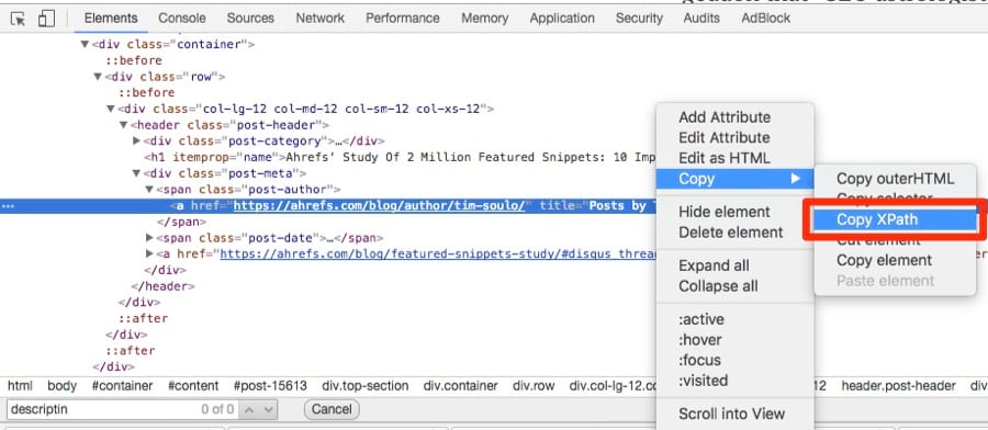
You can find the XPath for any element by doing the following (in Chrome):

Right-click > Inspect > Right-Click > Copy > Copy XPath

5. SEARCH strings for certain values

SEARCH lets you check whether or not a value exists in a string; it then returns the position at which the value is first found in the string.

Syntax: =SEARCH(search_query, text_to_search)

Here are some use cases:

• Check if a particular subdomain exists in URL (this is useful for bulk categorizing a list of URLs);
• Categorize keywords into various intent-based categories (e.g. branded, commercial, etc);
• Search for specific, undesirable characters within a URL;
• Search for certain words/phrases within a URL to categorize link prospects (e.g. “/category/guest-post”, “resources.html”, etc)

Let’s take a look at an example of SEARCH in action.

Here is a list of the top 300+ pages on Ahrefs.com (note: I used Site Explorer to gather this data):

All of the pages with /blog/ in the URL are blog posts. Let’s say that I wanted to tag each of these pages as “Blog post” during a content audit.

SEARCH (combined with an IF statement — this was discussed earlier in the guide) can do this in seconds; here’s the formula:

=IF(SEARCH("/blog/",A2),"YES","")

Let’s wrap it in an IFERROR and ARRAYFORMULA to neaten things up.

Here are a few other useful formulas:

• Find “write for us” pages in a list of URLs: =IF(SEARCH("/write-for-us/",A2),"Write for us page","");
• Find resource pages in a list of URLs: =IF(SEARCH("/resources.html",A2),"Resource page","");
• Find branded search terms (in a list of keywords): =IF(SEARCH("brand_name",A2),"Branded keyword","");
• Identify internal/external links (from a list of outbound links): =IF(SEARCH("yourdomain.com",A2),"Internal Link","External Link");

6. Import data from other spreadsheets using IMPORTRANGE

IMPORTRANGE allows you to import data from any other Google Sheet.

It doesn’t have to be on your Google Drive, either; it could belong to someone else (note: you will need permission to access the sheet if this is the case!)

Syntax: =IMPORTRANGE(spreadsheet_ID, range_to_import)

Here are a few use cases:

• Create client-facing sheets that piggyback off your “master” spreadsheet;
• Search and cross reference data across multiple Google Sheets (i.e. using IMPORTRANGE combined with VLOOKUPs);
• Pull in data from another sheet for use in a data validation;
• Pull in contact data from a “master” spreadsheet using VLOOKUPs

Let’s take a look at an example of IMPORTRANGE in action.

Here is a sheet with a list of hypothetical SEO clients + their budgets:

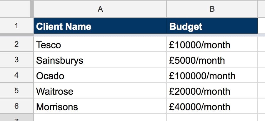
Let’s assume that I wanted to use this client list in another Google Sheet — I can import this entire data range using the following formula:

=IMPORTRANGE("SPREADSHEET_KEY","'SheetName'!A2:A")

Let’s also assume that you’re recording links built for these clients in a master spreadsheet; in one column you have the link URL and in the other, you want to record which client the link was for.

You can use IMPORTRANGE to create a dropdown of all clients using a data validation, like so:

This dropdown will self-update whenever you add/remove clients from your master spreadsheet.

7. QUERY data sets using SQL queries (this one is crazy powerful!)

QUERY is like VLOOKUP on steroids. It lets you query data using SQL, which allows you to get super-granular when it comes to data querying/retrieval.

Syntax: =QUERY(range, sql_query)

Here are a few use cases:

• Query a master link prospect database for specific prospects (e.g. find only prospects tagged as guest post opportunities, with a DR of above 50, and contact details present);
• Create super-granular client-facing documents that pull in data from a “master” spreadsheet;
• Query a massive on-site audit to pluck out only the pages that need attention.

Let’s go back to our sheet of tagged “blog posts”.

If we wanted to pull in all of the URLs that were tagged with “blog post” into a brand new spreadsheet, we could use this QUERY function:

=QUERY(DATA!A:B,"select A where B = 'Blog Post'")

But let’s say that we had a bigger data set. An export file from Site Explorer, perhaps.

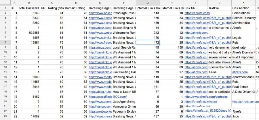
These export files can be quite data heavy, so let’s assume that we wanted to pull out a list of all referring pages with the following attributes:

• Dofollow link;
• DR > 50;
• Backlink status = active (i.e. not tagged as “removed”);
• External links count < 50;

Here’s the formula:

=QUERY('DATA - site explorer export'!A2:R,"SELECT E where D > 50 AND H < 50 AND M = 'Dofollow' AND N <> 'REMOVED'")

NOTE: It’s also possible to incorporate IMPORTRANGE into a QUERY function; this allows you to QUERY data from other sheets.

Final thoughts

Google Sheets is insanely powerful; this post only scratches the surface of what you can do with it.

I’d recommend playing around with the formulas above and seeing what you can come up with. I also recommend checking out the full library of Google Sheets formulas.

But, that’s still just the beginning: Google Sheets also integrates with Zapier and IFTTT, which means you can connect with hundreds of other tools and services, too.

And if you want to get really advanced, look into Apps Script—it’s crazy powerful!

If you have any creative uses for Google Sheets of your own, please let me know in the comments. I’d love to hear them!